Saving and Loading Data¶

Overview¶

In this section we discuss how to save and record measurement data with the MFIA Instrument using the LabOne user interface. In the LabOne user interface, there are 3 ways to save data:

Saving the data that is currently displayed in a plot
Continuously recording data in the background
Saving trace data in the History sub-tab

Furthermore, the History sub-tab supports loading data. In the following, we will explain these methods.

Saving Data from Plots¶

A quick way to save data from any plot is to click on the Save CSV icon at the bottom of the plot to store the currently displayed curves as a comma-separated value (CSV) file to the download folder of your web browser. Clicking on will save a graphics file instead.

Recording Data¶

The recording functionality allows you to store measurement data continuously, as well as to track instrument settings over time. The Config Tab gives you access to the main settings for this function. The Format selector defines which format is used: HDF5, CSV, or MATLAB. The CSV delimiter character can be changed in the User Preferences section. The default option is Semicolon. The Time Zone setting allows you to adjust the time stamps of the saved data.

The node tree display of the Record Data section allows you to browse through the different measurement data and instrument settings, and to select the ones you would like to record. For instance, the demodulator 1 measurement data is accessible under the path of the form Device 0000/Demodulators/Demod 1/Sample. An example for an instrument setting would be the filter time constant, accessible under the path Device 0000/Demodulators/Demod 1/Filter Time Constant.

The storage location is selected in the Drive drop-down menu of the Record section. The default location is the internal flash memory of the MFIA. Alternatively, you can plug an external USB drive into one of the USB Device ports on the back panel of the MFIA. If you do so, an additional option USB 1 or USB 2 appears in the Drive drop-down menu. If you’d like to save data directly to the host computer, you can install and run the LabOne Web Server on the host computer as described in Running LabOne on a Separate PC .

Note

Storing data on the internal flash memory is only recommended for occasional use, and for storing small amounts of data. The reason is that flash memories such as the one used in the instrument support only a finite number of write cycles and may wear out under heavy use. Storing data on the host computer (see Running LabOne on a Separate PC) or on an external USB hard drive is the safer alternative for such cases, and also offers higher speed.

Clicking on the Record checkbox will initiate the recording to the selected location. In case of demodulator and boxcar data, ensure that the corresponding data stream is enabled, as otherwise no data will be saved.

Figure 1: Browsing and inspecting files in the LabOne File Manager tab

In case HDF5 or MATLAB is selected as the file format, LabOne creates a single file containing the data for all selected nodes. For the CSV format, at least one file for each of the selected nodes is created from the start. At a configurable time interval, new data files are created, but the maximum size is capped at about 1 GB for easier data handling. The storage location is indicated in the Folder field of the Record Data section.

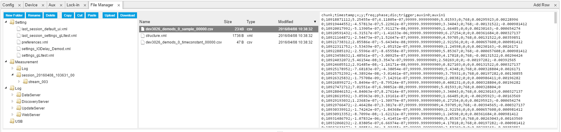
The File Manager Tab is a good place to inspect CSV data files. The file browser on the left of the tab allows you to navigate to the location of the data files and offers functionalities for managing files on the drive of the MF Instrument (or your computer’s drive in case you run the Web Server on the host computer). In addition, you can conveniently transfer files between the MFIA and the download folder on your host computer using the Upload/Download buttons. The file viewer on the right side of the tab displays the contents of text files up to a certain size limit. Figure 1 shows the Files tab after recording Demodulator Sample and Filter Time Constant for a few seconds. The file viewer shows the contents of the demodulator data file.

Note

The structure of files containing instrument settings and of those containing streamed data is the same. Streaming data files contain one line per sampling period, whereas in the case of instrument settings, the file usually only contains a few lines, one for each change in the settings. More information on the file structure can be found in the LabOne Programming Manual.

History List¶

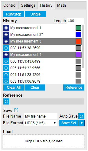
Tabs with a history list such as Sweeper Tab, Data Acquisition Tab , Scope Tab, Spectrum Analyzer Tab support feature saving, autosaving, and loading functionality. By default, the plot area in those tools displays the last 100 measurements (depending on the tool, these can be sweep traces, scope shots, DAQ data sets, or spectra), and each measurement is represented as an entry in the History sub-tab. The button to the left of each list entry controls the visibility of the corresponding trace in the plot; the button to the right controls the color of the trace. ¹Double-clicking on a list entry allows you to rename it. All measurements in the history list can be saved with . Clicking on the button (note the dropdown button ) saves only those traces that were selected by a mouse click. Use the Control or Shift button together with a mouse click to select multiple traces. The file location can be accessed by the Open Folder button . Figure 4.8 illustrates some of these features. Figure 2 illustrates the data loading feature.

Figure 2: History sub-tab features. The entries "My measurement 1" etc. were renamed by the user. Measurement 1, 2, 3, 4 are currently displayed in the plot because their left-hand-side button is enabled. Clicking on Save Sel would save "My measurement 3" and "My measurement 4" to a file, because these entries were selected (gray overlay) by a Control key + mouse click action.

Which quantities are saved depends on which signals have been added to the Vertical Axis Groups section in the Control sub-tab. Only data from demodulators with enabled Data Transfer in the Lock-in tab can be included in the files.

The history sub-tab supports an autosave functionality to store measurement results continuously while the tool is running. Autosave directories are differentiated from normal saved directories by the text "autosave" in the name, e.g. sweep_autosave_000. When running a tool continuously ( button) with Autosave activated, after the current measurement (history entry) is complete, all measurements in the history are saved. The same file is overwritten each time, which means that old measurements will be lost once the limit defined by the history Length setting has been reached. When performing single measurements ( button) with Autosave activated, after each measurement, the elements in the history list are saved in a new directory with an incrementing count, e.g. sweep_autosave_001, sweep_autosave_002.

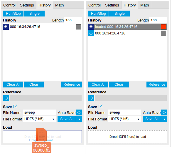
Data which was saved in HDF5 file format can be loaded back into the history list. Loaded traces are marked by a prefix "loaded " that is added to the history entry name in the user interface. The createdtimestamp information in the header data marks the time at which the data were measured.

Only files created by the Save button in the History sub-tab can be loaded.
Loading a file will add all history items saved in the file to the history list. Previous entries are kept in the list.
Data from the file is only displayed in the plot if it matches the current settings in the Vertical Axis Group section the tool. Loading e.g. PID data in the Sweeper will not be shown, unless it is selected in the Control sub-tab.
Files can only be loaded if the devices saving and loading data are of the same product family. The data path will be set according to the device ID loading the data.

Figure 3 illustrates the data loading feature.

Supported File Formats¶

HDF5¶

Hierarchical Data File 5 (HDF5) is a widespread memory-efficient, structured, binary, open file format. Data in this format can be inspected using the dedicated viewer HDFview. HDF5 libraries or import tools are available for Python, MATLAB, LabVIEW, C, R, Octave, Origin, Igor Pro, and others. The following example illustrates how to access demodulator data from a sweep using the h5py library in Python:

import h5py
filename = 'sweep_00000.h5'
f = h5py.File(filename, 'r')
x = f['000/dev3025/demods/0/sample/frequency']

The data loading feature of LabOne supports HDF5 files, while it is unavailable for other formats.

MATLAB¶

The MATLAB File Format (.mat) is a proprietary file format from MathWorks based on the open HDF5 file format. It has thus similar properties as the HDF5 format, but the support for importing .mat files into third-party software other than MATLAB is usually less good than that for importing HDF5 files.

SXM¶

SXM is a proprietary file format by Nanonis used for SPM measurements.

ZView¶

ZView is a comma-separated value format adapted for impedance analysis and supported by the analysis software with the same name by Scribner Associates. Since there are many variants of this structure in use by other impedance modeling software tools, LabOne allows you to adapt the ZView format to your preferred standard using a template file. Proceed as follows:

In the Config Tab, select ZView as Format setting for data recording.
Enable and disable the Record checkbox. This step is only needed the first time you use the ZView format and creates a default template file.
Open the File Manager Tab and look for the file savefile_template.txt in the Setting folder. Use the Download button to transfer it to your PC, and modify it according to your needs (see below).
Use the Upload button to transfer the modified file (with the same name savefile_template.txt) back into the Setting folder.

Any successive data recording in ZView format will adhere to this new template. The last line of the template file defines the data row format of the saved data file and is repeated for each sample. Everything above the last line defines the data file header and is written to the data file a single time. Both in the header part and in the last line, keywords of the form ${variable} are replaced by the respective quantity or setting. Any other text in the template file is written verbatim to the data file.

The following tables list the keywords supported in the header part and in the last line of the template file.

Table 1: Keywords supported in the header part of the ZView template file
Keyword	Datum
`${year}, ${month}, ${day}, ${hours}, ${minutes}, ${seconds}`	Respective component of the current time stamp
`${month_str}`	Abbreviated month name (Jan, Feb, Mar, ...)
`${numpoints}`	Number of recorded data samples
`${filename}`	File name
`${grid_columns}`	Number of columns in Data Acquisition Tab
`${grid_rows}`	Number of rows in Data Acquisition Tab
`${grid_mode}`	Mode setting in Data Acquisition Tab (nearest, linear, Lanczos)
`${grid_operation}`	Operation setting in Data Acquisition Tab (replace, average)
`${grid_scan_direction}`	Scan direction in Data Acquisition Tab (forward, reverse, bidirectional)
`${grid_repetitions}`	Repetitions setting in Data Acquisition Tab

Table 2: Keywords supported in the last line of the ZView template file
Keyword	Datum
`${frequency}`	Measurement frequency
`${phasez}`	Impedance complex phase
`${absz}`	Impedance absolute value
`${realz}`	Impedance real part
`${imagz}`	Impedance imaginary part
`${param0}`	Representation parameter 1
`${param1}`	Representation parameter 2
`${drive}`	Drive voltage amplitude
`${bias}`	DC bias voltage
`${timestamp}`	Measurement time in units of the instrument clock period
`${time_sec}`	Time in seconds relative to first sample
`${count}`	Successive sample count
`${flags}`	Integer containing bit flags for confidence indicators and device state information (see )

Bit number	Condition
0	Internal calibration is enabled
1	User compensation is enabled
2...3	Reserved
4	Confidence indicator: overflow on voltage signal input
5	Confidence indicator: overflow on current signal input
6	Confidence indicator: underflow on voltage signal input
7	Confidence indicator: underflow on current signal input
8...10	Reserved
11	Confidence indicator: Z too low for 2-terminal
12	Confidence indicator: suppression of first representation parameter (PARAM0)
13	Confidence indicator: suppression of second representation parameter (PARAM1)
14	Reserved
15	Confidence indicator: frequency limit of current input exceeded
16	Confidence indicator: strong compensation detected on first representation parameter (PARAM0)
17	Confidence indicator: strong compensation detected on second representation parameter (PARAM1)
18...23	Reserved
24	Confidence indicator: open detected
25...31	Reserved

Bit assignment in ${flags} data column

LabOne Net Link¶

Measurement and cursor data can be downloaded from the browser as CSV data. This allows for further processing in any application that supports CSV file formats. As the data is stored internally on the web server it can be read by direct server access from other applications. Most up-to-date software supports data import from web pages or CSV files over the internet. This allows for automatic import and refresh of data sets in many applications. To perform the import the application needs to know the address from where to load the data. This link is supplied by the LabOne User Interface. The following chapter lists examples of how to import data into some commonly used applications.

The CSV data sent to the application is a snap-shot of the data set on the web server at the time of the request. Many applications support either manual or periodic refresh functionality.

Since tabs can be instantiated several times within the same user interface, the link is specific to the tab that it is taken from. Changing the session on the LabOne User Interface or removing tabs may invalidate the link.

Supported applications:

Excel
MATLAB
Python
C#.NET
Igor Pro
Origin

Excel¶

These instructions are for Excel 2010 (English). The procedure for other versions may differ.

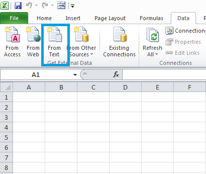
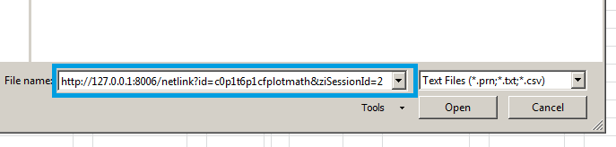
In Excel, click on the cell where the data is to be placed. From the Data ribbon, click the "From Text" icon. The "Import Text File" dialog will appear.
In LabOne, click the "Link" button of the appropriate Math tab. Copy the selected text from the "LabOne Net Link" dialog to the clipboard (either with Ctrl-C or by right clicking and selecting "Copy").
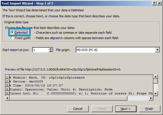
In Excel, paste the link into the "File name" entry field of the "Import Text File" dialog and click the "Open" button. This will start the text import wizard. Ensure that the "Delimited" button is checked before clicking the "Next" button.
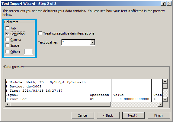
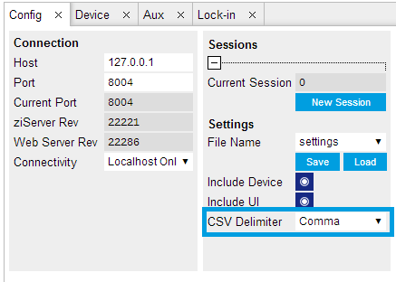
In the next dialog, select the delimiter character corresponding to that selected in LabOne (this can be found in the "Sessions" section of the Config tab). The default is semicolon. Click the "Next" button.
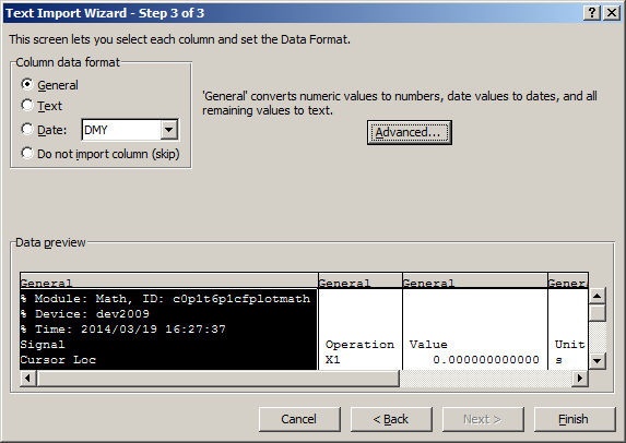
In the next dialog, click on "Finish" and then "OK" in the "Import Data" dialog. The data from the Math tab will now appear in the Excel sheet.
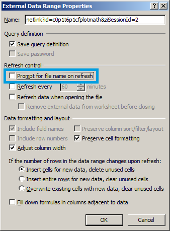
The data in the sheet can be updated by clicking the "Refresh All" icon. To make updating the data easier, the "Import text file" dialog can be suppressed by clicking on "Properties".
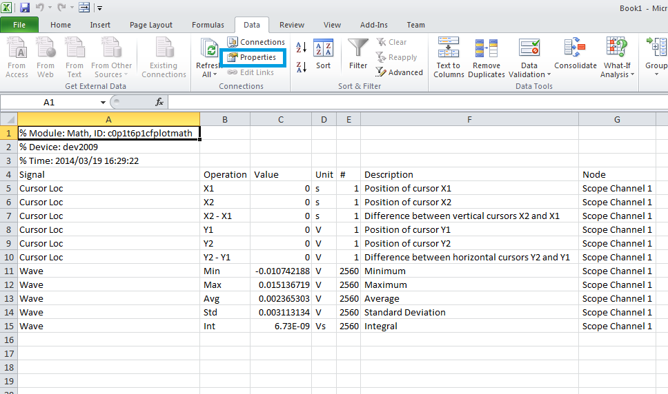
Deactivate the check box "Prompt for file name on refresh".

MATLAB¶

By copying the link text from the "LabOne Net Link" dialog to the clipboard, the following code snippet can be used in MATLAB to read the data.

textscan(urlread(clipboard('paste')),'%s%s%f%s%d%s%s','Headerlines', 4,'Delimiter', ';')

Python¶

The following code snippet can be used in Python 2 to read the LabOne Net Link data, where "url" is assigned to the text copied from the "LabOne Net Link" dialog.

import csv
import urllib2
url = "http://127.0.0.1:8006/netlink?id=c0p5t6p1cfplotmath&ziSessionId=0"
webpage = urllib2.urlopen(url)
datareader = csv.reader(webpage)
data = []
for row in datareader:
    data.append(row)

C#.NET¶

The .NET Framework offers a WebClient object which can be used to send web requests to the LabOne WebServer and download LabOne Net Link data. The string with comma separated content can be parsed by splitting the data at comma borders.

using System;
using System.Text;
using System.Net;

namespace ExampleCSV
{
  class Program
  {
    static void Main(string[] args)
    {
      try
      {
        WebClient wc = new WebClient();
        byte[] buffer = wc.DownloadData("http://127.0.0.1:8006/netlink?id=c0p1t6p1cfplotmath&ziSessionId=0");
        String doc = Encoding.ASCII.GetString(buffer);
        // Parse here CSV lines and extract data
        // ...
        Console.WriteLine(doc);
      } catch (Exception e) {
        Console.WriteLine("Caught exception: " + e.Message);
      }
    }
  }
 }

Igor Pro¶

These instructions are for Igor Pro 6.34A English. The procedure for other versions may differ.

For Igor Pro, the CSV separator has to be the comma. Set this in the LabOne Config tab as follows:
In Igor Pro, select the menu "Data→Load Waves→Load Waves...".
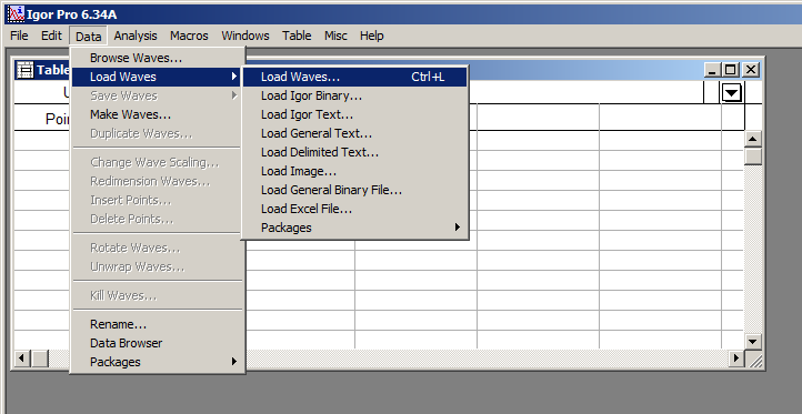
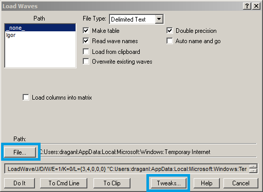
In the "Load Waves" dialog, click the "File..." button and paste the link text from the "LabOne Net Link" dialog into the entry field. Then click the "Tweaks..." button to open the "Load Data Tweaks" dialog.
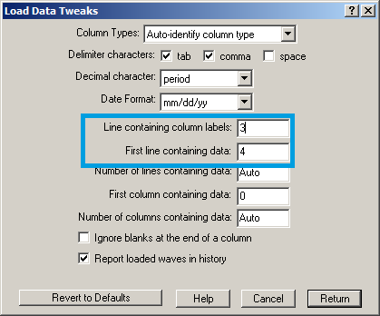
Adjust values as highlighted below and click "Return". The "Loading Delimited Data" dialog will appear.
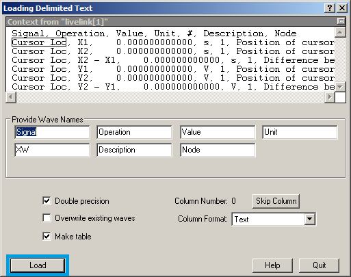
Click the "Load" button to read the data.
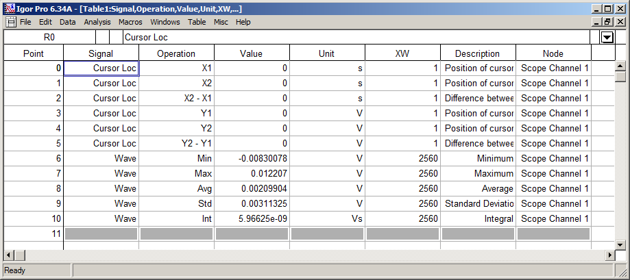
The data will appear in the Igor Pro main window.

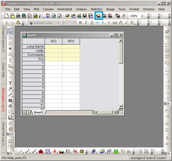
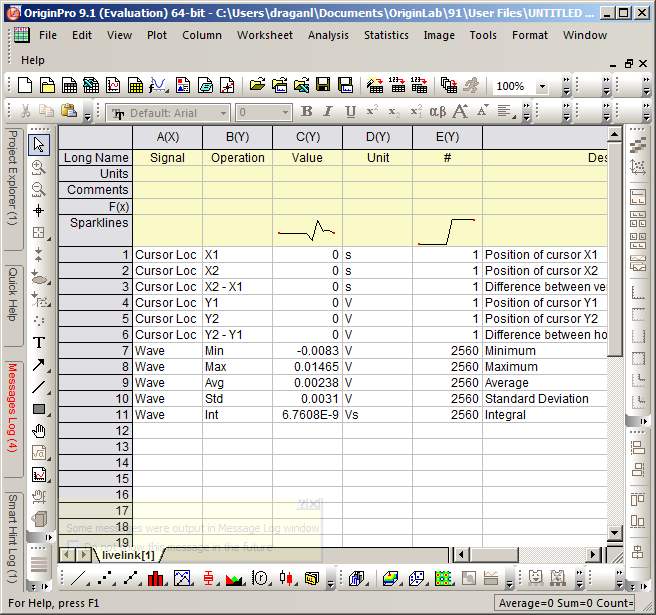
Origin¶

These instructions are for Origin 9.1 English. The procedure for other versions may differ.

Open the import wizard by clicking on the icon highlighted below.
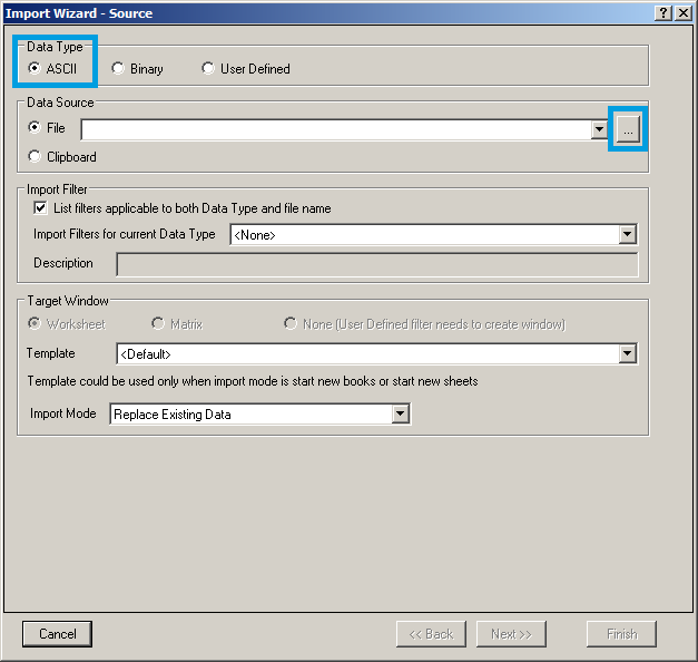
Ensure that the ASCII button is selected. Click the "..." button. See screenshot below. The "Import Multiple ASCII" dialog will appear.
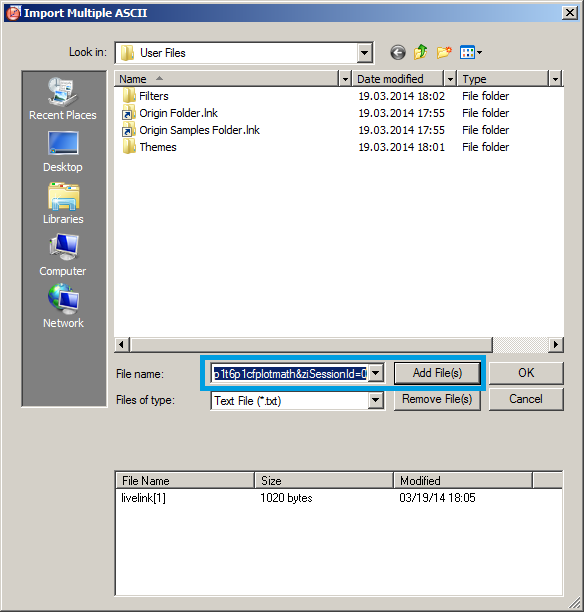
Paste the link text from the "LabOne Net Link" dialog into the entry field highlighted below. Then click "Add File(s)" followed by "OK".
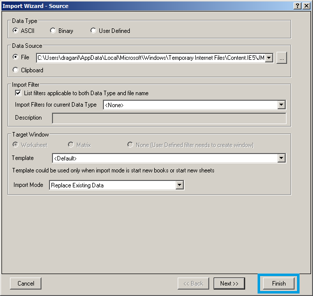
Back in the "Import Wizard - Source" dialog click "Finish".
The data will appear in the Origin main window.

Among the mentioned tools, the Scope is exceptional: it displays the most recent acquisition, and its display color is fixed. However, the Persistence feature represents a more specialized functionality for multi-trace display. ↩