Quantum Analyzer Setup Tab
The Quantum Analyzer Setup is the main control panel for the qubit measurement unit on the instrument (see functional overview for an overview block diagram). It is available on all UHFQA instruments.
Features
- Raw signal deskew
- Signal rotation in I/Q plane
- 10×10 crosstalk subpression matrix
- Threshold operation
- Qubit-qubit correlation analysis
Description
| Control/Tool | Option/Range | Description |
|---|---|---|
| QA Setup | Configure the Qubit Measurement Unit |
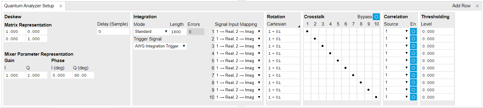
The Quantum Analyzer Setup tab (see LabOne UI: Quantum Analyzer Setup tab) is divided into different sections each representing a signal processing step starting from raw signal deskew to the final threshold operation that transforms an analog I/Q signal into a discrete qubit state. This tab represents the interface to the following functional blocks: the integration units, the internal oscillator, the crosstalk subpression matrix, the deskew matrix, the correlation unit, the statistics unit, and the thesholding unit. A block diagram representing the flow of data and trigger signals between the functional blocks is found in Architecture and Signalling.
Two-element vectors of samples arrive at 1.8 GSa/s from Signal Inputs 1 and 2. In the Deskew section, at this rate, each sample vector is multiplied by a 2×2 Rotation/Gain matrix. The default value is the identity matrix [1, 0; 0, 1] which leaves both input signals unchanged. Changing this to a different value allows the user to compensate for signal imperfections such as analog linear crosstalk, or mixer amplitude imbalance.
In the Integration section, each of the two input signals is demodulated by multiplying with a reference signal and the product is integrated over a fixed time T after reception of a trigger. The user can choose the mode of operation of the weighted integration. In Standard mode, the reference signal is given by the Integration Weights programmed to the instrument memory using the Quantum Analyzer Input Tab. This mode offers the full flexibility to define a custom integration weight to realize a matched filter. In Spectroscopy mode, the reference signal is given by sine and cosine signals generated by the internal digital oscillator controlled from the Inputs/Outputs Tab, which allows for longer integration times and thus higher frequency resolution than the Standard mode. The input signals VSig In 1(t) and VSig In 2(t) of duration T are reduced to a single pair of voltages VI and VQ. Since there are 10 separate qubit measurement units, there can be up to 10 pairs (VI, q, VQ, q for q=1...10), each corresponding to one frequency component of the signals V{Sig In 1}(t) and V{Sig In 2}(t).
The Rotation section rotates and scales the signal in the complex plane after integration. For each of the 10 channels, the rotation is characterized by a complex number zq = xq+iyq = rq×exp(iθq). The demodulated signal is multiplied with zq: V'I, q + iV'{Q, q} = (V{I, q} + iV{Q, q})×zq. The user may specify zq in polar coordinates in the form "r @ θ" or in Cartesian coordinates in the form "x + y i". Examples are "1@45" for a 45 degree rotation, or "0.0 + 1.0 i" for a 90 degree rotation. The purpose of the rotation step is to ensure that the readout contrast is shifted into the in-phase signal component, i.e., that the state of qubit q only affects V'{I, q} but not V'{Q, q}.
The Crosstalk section is a graphical representation of the 10×10 crosstalk subpression matrix C that subports systematic minimization of the influence of one qubit’s state on another qubit’s readout signal. The signal processing up to after the rotation step can be abstracted as a 10×10 matrix M that transforms the vector of qubit states (s1,...,s10), with sq = 0 or 1, into the vector of signals (V'{I, 1}, ... V'{I, 10}). This matrix can be measured systematically by preparing the qubit system in different states of the form (0,..., 0, 1, 0,..., 0), and measuring the resulting signal. Using the Crosstalk Suppression optimally relies on finding the matrix C such that C×M is diagonal. Due to the complexity of this method, setting the elements of the crosstalk subpression matrix C from the graphical UI would be impractical, and its elements can only be set from the API. We denote the signals after crosstalk subpression with a double prime as (V''{I, 1}, ... V''{I, 10}) = C×(V'{I, 1}, ... V'{I, 10}).
The Correlation section optionally enables the outputs of two readout channels to be multiplied prior to averaging, logging, etc. When enabled, the corresponding channel is multiplied with another channel selected as the Source.
The Thresholds section allows one to define a voltage threshold to transform the in-phase quadrature V''{I, q} of the readout signal into a discrete qubit state, 0 or 1.
Functional Elements
| Control/Tool | Option/Range | Description |
|---|---|---|
| Rotation/Gain Matrix | Implements a 2×2 matrix multiplication. The two input signals are treated as a vector with two elements and the result is a vector as well. | |
| In-Phase Gain | Gain of in-phase branch | |
| Quadrature Gain | Gain of quadrature branch | |
| In-Phase Phase | Phase of in-phase branch | |
| Quadrature Phase | Phase of quadrature branch | |
| Mode | Application mode. | |
| Standard | The integration weights are given by the user-programmed filter memory. | |
| Spectroscopy | The integration weights are generated by a digital oscillator. This mode offers enhanced frequency resolution. | |
| Readout Trigger Selection | Select the source for triggering the readout. | |
| Trigger Input 1 | Use the Trigger Input 1 as the trigger signal. | |
| Trigger Input 2 | Use the Trigger Input 2 as the trigger signal. | |
| Trigger Input 3 | Use the Trigger Input 3 as the trigger signal. | |
| Trigger Input 4 | Use the Trigger Input 4 as the trigger signal. | |
| AWG Integration Trigger | Use the AWG Integration Trigger as the trigger signal. | |
| Spectroscopy Trigger Selection | Selects the source for triggering the spectroscopy. | |
| Clear | Empty all Integration Weights memory slots. | |
| Integration Length | The integration time of all weighted integration units specified in units of samples. In Standard mode, a maximum of 4096 samples can be integrated, which corresponds to 2.3 µs. In Spectroscopy mode, a maximum of 16.7 MSa can be integrated, which corresponds to ~10 ms. | |
| Errors | Number of hold-off violations detected in the INTEGRATION unit since last reset. | |
| Delay | A delay time in units of samples that adjusts the time at which the integration starts in relation to the trigger signal of the weighted integration units. | |
| Source | Controls the routing of the input signals to the INTEGRATION units. | |
| 1 -> Real, 2 -> Imag | Signal input 1 to real part, Signal input 2 to imaginary part. | |
| 2 -> Real, 1 -> Imag | Signal input 2 to real part, Signal input 1 to imaginary part. | |
| 1 -> Real, 1 -> Imag | Signal input 1 to real part, Signal input 1 to imaginary part. | |
| 2 -> Real, 2 -> Imag | Signal input 2 to real part, Signal input 2 to imaginary part. | |
| Rotation | Complex rotation coefficient applied to the signals after integration. | |
| Representation | Select between Cartesian and polar representation of the complex rotation coefficient. Cartesian coordinates are entered in the format "x+iy", polar coordinates in the format "r@a" where x, y, r, and a are real numbers. | |
| Crosstalk | Graphical representation of the 10×10 crosstalk suppression matrix. Positive values are black, negative values are red. | |
| Bypass Crosstalk | Bypass the Crosstalk matrix in order to reduce the latency through the system. | |
| Bypass Rotation | Bypass Rotation in order to reduce the latency through the system. | |
| Bypass Deskew | Bypass Deskew in order to reduce the latency through the system. | |
| En | Enable the correlation mode for the given channel. | |
| Source | Controls the channel with which correlation should be made. Selecting the same channel as the readout channel number corresponds to self-correlation. | |
| Level | The discretization level applied to the output of the Crosstalk Suppression matrix. | |
| Length | Sets the integration length in spectroscopy mode in number of samples. A maximum of 33.5 MSa (2^25 samples) can be integrated, which corresponds to 16.7 ms. | |
| Delay | Sets the delay of the start of the integration in spectroscopy mode with respect to the Trigger Signal. | |
| PSD Enable | Enable the power spectral density mode of the spectroscopy mode. | |
| Offset Frequency | Sets the digital oscillator frequency. The sum of the Offset Frequency and the Center Frequency correspond to the frequency of the microwave tone at the Out connector. | |
| Output Frequency | Displays the carrier frequency of the microwave signal at the Out connector. This frequency corresponds to the sum of the Center Frequency and the Offset Frequency. | |
| Amplitude | Amplitude of the microwave signal relative to the range of the Output. | |
| Set Mode | Set Generator Waveform by parametric generation or CSV Upload. | |
| Parametric | Generator Waveform are generated by defining sine wave parameters. | |
| Upload | Generator Waveform are uploaded by the user in a form of a CSV file. | |
| Frequency | Frequency of the complex exponential function. | |
| Phase | Phase of the complex exponential function. | |
| Window Type | Window function to be applied to the complex exponential function. | |
| Window Length | Length of the selected window in samples, starting from 0. | |
| Waveform Memory | Selects the waveform memory for parametric or arbitrary waveform upload. | |
| Set To device | Write the real and imaginary part of the Waveform to the selected Waveform Memory. | |
| Set To Device | Write the real and imaginary part of the Waveform to the selected Waveform Memory. | |
| CSV File | Drag and drop CSV file containing columns of Sequencer Waveform. | |
| Amplitude | Amplitude of the complex exponential function. | |
| Clear | Empty all Readout Waveform memory slots. | |
| Sequencer | Runs the Sequencer. | |
| Status | grey/green/yellow/red | Displays the status of the sequencer on the instrument. Off: Ready, not running. Green: Running, not waiting for any trigger event. Yellow: Running, waiting for a trigger event. Red: Not ready (e.g., pending elf upload, no elf uploaded) |
| Enable | If enabled, the waveforms and integration weights get modulated with the oscillators. | |
| Frequency | Controls the frequency of each digital Oscillator. | |
| Gain | Controls the gain of each digital Oscillator. The gain is defined relative to the Output Range of the Readout Channel. | |
| Enable | Enables the waveform hold functionality. | |
| Start Index | Index of the waveform sample where to hold the playback. | |
| Length | Duration in number of samples for which to hold the playback. | |
| Downsampling Factor | Down-sampling factor for integration weights. Setting the factor to 1 means no downsampling. |