Sweeper Tab
The Sweeper is a highly versatile measurement tool available on all UHFLI instruments. The Sweeper enables scans of an instrument parameter over a defined range and simultaneous measurement of a selection of continuously streamed data. In the special case where the sweep parameter is an oscillator frequency, the Sweeper offers the functionality of a frequency response analyzer (FRA), a well-known class of instruments. On UHFAWG instruments, the tab is available if at least one of the options UHF-BOX, UHF-CNT, or UHF-LIA is installed.
Features
- Full-featured parametric sweep tool for frequency, phase shift, output amplitude, DC output voltages, etc.
- Simultaneous display of data from different sources (Demodulators, PIDs, auxiliary inputs, and others)
- Different application modes, e.g. Frequency response analyzer (Bode plots), noise amplitude sweeps, etc.
- Different sweep types: single, continuous (run / stop), bidirectional, binary
- Persistent display of previous sweep results
- XY Mode for Nyquist plots or I-V curves
- Normalization of sweeps
- Auto bandwidth, averaging and display normalization
- Support for Input Scaling and Input Units
- Phase unwrap
- Full support of sinc filter
Description
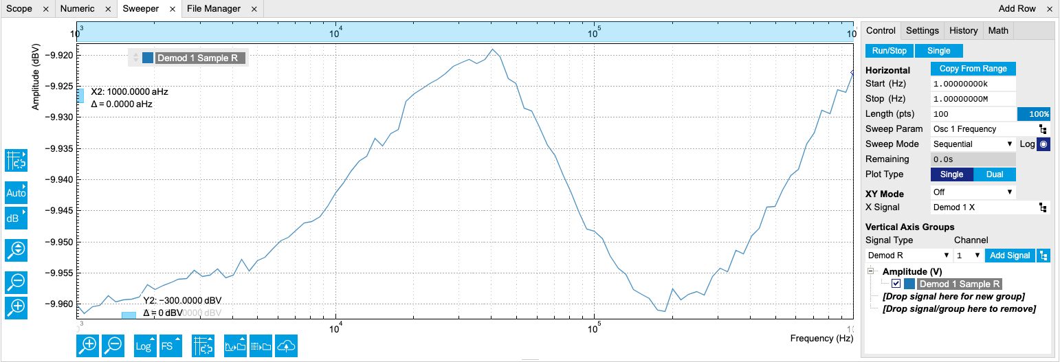
The Sweeper supports a variety of experiments where a parameter is changed stepwise and numerous measurement data can be graphically displayed. Open the tool by clicking the corresponding icon in the UI side bar. The Sweeper tab (see Figure 1) is divided into a plot section on the left and a configuration section on the right. The configuration section is further divided into a number of sub-tabs.
| Control/Tool | Option/Range | Description |
|---|---|---|
| Sweeper | Sweep frequencies, voltages, and other quantities over a defined range and display various response functions including statistical operations. |
The Control sub-tab holds the basic measurement settings such as Sweep Parameter, Start/Stop values, and number of points (Length) in the Horizontal section. Measurement signals can be added in the Vertical Axis Groups section. A typical use of the Sweeper is to perform a frequency sweep and measure the response of the device under test in the form of a Bode plot. As an example, AFM and MEMS users require to determine the resonance frequency and the phase delay of their oscillators. The Sweeper can also be used to sweep parameters other than frequency, for instance signal amplitudes and DC offset voltages. A sweep of the Auxiliary Output offset can for instance be used to measure current-voltage (I-V) characteristics. The XY Mode allows one to use a measured signal, rather than the sweep parameter, on the horizontal axis. This is useful to obtain Nyquist plots in impedance measurements, or to display an I-V curve in a four-probe measurement of a nonlinear device.
For frequency sweeps, the sweep points are distributed logarithmically, rather than linearly, between the start and stop values by default. This feature is particularly useful for sweeps over several decades and can be disabled with the Log checkbox. The Sweep Mode setting is useful for identifying measurement problems caused by hysteretic sample behavior or too fast sweeping speed. Such problems would cause non-overlapping curves in a bidirectional sweep.
Note
The Sweeper actively modifies the main settings of the demodulators and oscillators. So in particular for situations where multiple experiments are served maybe even from different control computers great care needs to be taken so that the parameters altered by the sweeper module do not have unwanted effects elsewhere.
The Sweeper offers two operation modes differing in the level of detail of the accessible settings: the Application Mode and the Advanced Mode. Both of them are accessible in the Settings sub-tab. The Application Mode provides the choice between six measurement approaches that should help to quickly obtain correct measurement results for a large range of applications. Users who like to be in control of all the settings can access them by switching to the Advanced Mode.
In the Statistics section of the Advanced Mode one can control how data is averaged at each sweep point: either by specifying the Sample count, or by specifying the number of filter time constants (TC). The actual measurement time is determined by the larger of the two settings, taking into account the demodulator sample rate and filter settings. The Algorithm settings determines the statistics calculated from the measured data: the average for general purposes, the deviation for noise measurements, or the mean square for power measurements. The Phase Unwrap features ensures continuity of a phase measurement curve across the PM180 degree boundary. Enabling the Sinc Filter setting means that the demodulator Sinc Filter gets activated for sweep points below 50 Hz in Auto and Fixed mode. This speeds up measurements at small frequencies as explained in the Sinc Filtering .
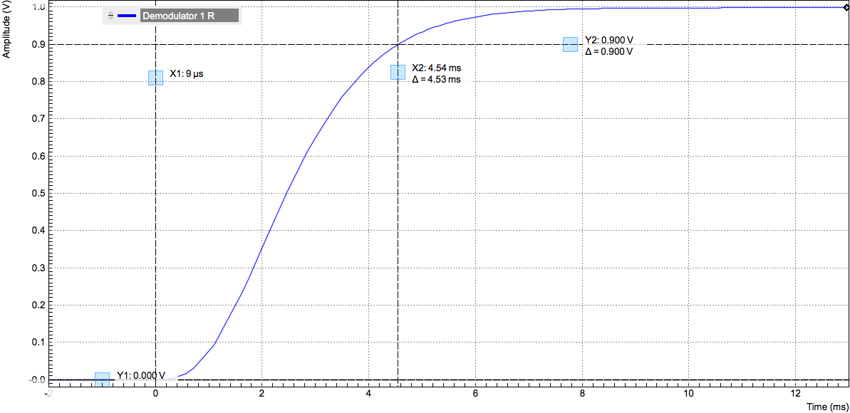
In the Settling section one can control the waiting time between a parameter setting and the first measurement. Similarly to the Statistics setting, one has the choice between two different representations of this waiting time. The actual settling time is the maximum of the values set in units of absolute time and a time derived from the demodulator filter and a desired inaccuracy (e.g. 1 m for 0.1%). Let’s consider an example. For a 4th order filter and a 3 dB bandwidth of 100 Hz we obtain a step response the attains 90% after about 4.5 ms. This can be easily measured by using the Data Acquisition tool as indicated in Figure 2. It is also explained in Discrete-Time Filters. In case the full range is set to 1 V this means a measurement has a maximum error caused by imperfect settling of about 0.1 V. However, for most measurements the neighboring values are close compared to the full range and hence the real error caused is usually much smaller.
In the Filter section of the Advanced mode, the Bandwidth Mode setting determines how the filters of the activated demodulators are configured. In Manual mode, the current setting (in the Lock-in tab) remains unchanged by the Sweeper. In Fixed mode, the filter settings can be controlled from within the Sweeper tab. In Auto mode, the Sweeper determines the filter bandwidth for each sweep point based on a desired ω suppression. The ω suppression depends on the measurement frequency and the filter steepness. For frequency sweeps, the bandwidth will be adjusted for every sweep point within the bound set by the Max Bandwidth setting. The Auto mode is particularly useful for frequency sweeps over several decades, because the continuous adjustment of the bandwidth considerably reduces the overall measurement time.
By default the plot area keeps the memory and display of the last 100
sweeps represented in a list in the History sub-tab. See History
List
for more details on how data in the history list can be managed and
stored. With the Reference feature, it is possible to divide all
measurements in the history by a reference measurement. This is useful
for instance to eliminate spurious effects in a frequency response
sweep. To define a certain measurement as the reference, mark it in the
list and click on  .
Then enable the Reference mode with the checkbox below the list to
update the plot display. Note that the Reference setting does not affect
data saving: saved files always contain raw data.
.
Then enable the Reference mode with the checkbox below the list to
update the plot display. Note that the Reference setting does not affect
data saving: saved files always contain raw data.
Note
The Sweeper can get stuck whenever it does not receive any data. A common mistake is to select to display demodulator data without enabling the data transfer of the associated demodulator in the Lock-in tab.
Note
Once a sweep is performed the sweeper stores all data from the enabled demodulators and auxiliary inputs even when they are not displayed immediately in the plot area. These data can be accessed at a later point in time simply by choosing the corresponding signal display settings (Input Channel).
Functional Elements
| Control/Tool | Option/Range | Description |
|---|---|---|
| Run/Stop |  |
Runs the sweeper continuously. |
| Single |  |
Runs the sweeper once. |
| Copy From X-Axis | Takes over start and stop value from the X-axis. | |
| Copy From X-Cursors | Takes over start and stop value from X-cursors. Button is disabled when one or both X cursors are not visible. | |
| Start (unit) | numeric value | Start value of the sweep parameter. The unit adapts according to the selected sweep parameter. |
| Stop (unit) | numeric value | Stop value of the sweep parameter. The unit adapts according to the selected sweep parameter. |
| Length | integer value | Sets the number of measurement points. |
| Progress | 0 to 100% | Reports the sweep progress as ratio of points recorded. |
| Sweep Param |  |
Selects the parameter to be swept. Navigate through the tree view that appears and click on the required parameter. The available selection depends on the configuration of the device. |
| Sweep Mode | Select the scanning type, default is sequential (incremental scanning from start to stop value) | |
| Sequential | Sequential sweep from Start to Stop value | |
| Binary | Non-sequential sweep continues increase of resolution over entire range | |
| Bidirectional | Sequential sweep from Start to Stop value and back to Start again | |
| Reverse | Reverse sweep from Stop to Start value | |
| X Distribution | Linear / Logarithmic | Selects between linear and logarithmic distribution of the sweep parameter. |
| Remaining | numeric value | Reporting of the remaining time of the current sweep. A valid number is only displayed once the sweeper has been started. An undefined sweep time is indicated as NaN. |
| Invert Y Axis | ON / OFF | The xy-plot is displayed with inverted y-axis. This mode is used for Nyquist plots that allow for displaying -imag(z) on the y-axis and real(z) on the x-axis. |
| X Signal | |
Selects the signal that defines the x-axis for xy-plots. The available selection depends on the configuration of the device. Displaying the selected signal source will result in a diagonal straight line. |
For the Vertical Axis Groups, please see the table "Vertical Axis Groups description" in the section called "Vertical Axis Groups".
| Control/Tool | Option/Range | Description |
|---|---|---|
| Filter | Application Mode: preset configuration. Advanced Mode: manual configuration. | |
| Application Mode | The sweeper sets the filters and other parameters automatically. | |
| Advanced Mode | The sweeper uses manually configured parameters. | |
| Application | Select the sweep application mode | |
| Parameter Sweep | Only one data sample is acquired per sweeper point. | |
| Parameter Sweep Averaged | Multiple data samples are acquired per sweeper point of which the average value is displayed. | |
| Noise Amplitude Sweep | Multiple data samples are acquired per sweeper point of which the standard deviation is displayed (e.g. to determine input noise). For accurate noise measurement, the signal amplitude R is replaced by its quadrature components X and Y. | |
| Freq Response Analyzer | Narrow band frequency response analysis. Averaging is enabled. | |
| 3-Omega Sweep | Optimized parameters for 3-omega application. Averaging is enabled. | |
| FRA (Sinc Filter) | The sinc filter helps to speed up measurements for frequencies below 50 Hz in FRA mode. For higher frequencies it is automatically disabled. Averaging is off. | |
| Impedance | This application mode uses narrow bandwidth filter settings to achieve high calibration accuracy. | |
| Precision | Choose between a high speed scan speed or high precision and accuracy. | |
| Low -> fast sweep | Medium accuracy/precision is optimized for sweep speed. | |
| High -> standard speed | Medium accuracy/precision takes more measurement time. | |
| Very high -> slow sweep | High accuracy/precision takes more measurement time. | |
| Bandwidth Mode | Automatically is recommended in particular for logarithmic sweeps and assures the whole spectrum is covered. | |
| Auto | All bandwidth settings of the chosen demodulators are automatically adjusted. For logarithmic sweeps the measurement bandwidth is adjusted throughout the measurement. | |
| Fixed | Define a certain bandwidth which is taken for all chosen demodulators for the course of the measurement. | |
| Manual | The sweeper module leaves the demodulator bandwidth settings entirely untouched. | |
| Time Constant/Bandwidth Select | Defines the display unit of the low-pass filter to use for the sweep in fixed bandwidth mode: time constant (TC), noise equivalent power bandwidth (NEP), 3 dB bandwidth (3 dB). | |
| TC | Defines the low-pass filter characteristic using time constant of the filter. | |
| Bandwidth NEP | Defines the low-pass filter characteristic using the noise equivalent power bandwidth of the filter. | |
| Bandwidth 3 dB | Defines the low-pass filter characteristic using the cut-off frequency of the filter. | |
| Time Constant/Bandwidth | numeric value | Defines the measurement bandwidth for Fixed bandwidth sweep mode, and corresponds to either noise equivalent power bandwidth (NEP), time constant (TC) or 3 dB bandwidth (3 dB) depending on selection. |
| Order | numeric value | Selects the filter roll off to set on the device in Fixed and Auto bandwidth modes. It ranges from 1 (6 dB/octave) to 8 (48 dB/octave). |
| Max Bandwidth (Hz) | numeric value | Maximal bandwidth used in auto bandwidth mode. The effective bandwidth will be calculated based on this max value, the frequency step size, and the omega suppression. The noise-equivalent power (NEP) is correctly taken into account for demodulation bandwidths of up to 1.25 MHz. |
| BW Overlap | ON / OFF | If enabled the bandwidth of a sweep point may overlap with the frequency of neighboring sweep points. The effective bandwidth is only limited by the maximal bandwidth setting and omega suppression. As a result, the bandwidth is independent of the number of sweep points. For frequency response analysis bandwidth overlap should be enabled to achieve maximal sweep speed. |
| Omega Suppression (dB) | numeric value | Suppression of the omega and 2-omega components. Large suppression will have a significant impact on sweep time especially for low filter orders. |
| Min Settling Time (s) | numeric value | Minimum wait time in seconds between a sweep parameter change and the recording of the next sweep point. This parameter can be used to define the required settling time of the experimental setup. The effective wait time is the maximum of this value and the demodulator filter settling time determined from the Inaccuracy value specified. |
| Inaccuracy | numeric value | Demodulator filter settling inaccuracy defining the wait time between a sweep parameter change and recording of the next sweep point. The settling time is calculated as the time required to attain the specified remaining proportion [1e-13, 0.1] of an incoming step function. Typical inaccuracy values: 10 m for highest sweep speed for large signals, 100 u for precise amplitude measurements, 100 n for precise noise measurements. Depending on the order the settling accuracy will define the number of filter time constants the sweeper has to wait. The maximum between this value and the settling time is taken as wait time until the next sweep point is recorded. |
| Settling Time (TC) | numeric value | Calculated wait time expressed in time constants defined by the specified filter settling inaccuracy. |
| Algorithm | Selects the measurement method. | |
| Averaging | Calculates the average on each data set. | |
| Standard Deviation | Calculates the standard deviation on each data set. | |
| Average Power | Calculates the electric power based on a 50 Ω input impedance. | |
| Count (Sa) | integer number | Sets the number of data samples per sweeper parameter point that is considered in the measurement. The maximum between samples, time and number of time constants is taken as effective calculation time. |
| Count (s) | numeric value | Sets the time during which data samples are processed. The maximum between samples, time and number of time constants is taken as effective calculation time. |
| Count (TC) | 0/5/15/50/100 TC | Sets the effective measurement time per sweeper parameter point that is considered in the measurement. The maximum between samples, time and number of time constants is taken as effective calculation time. |
| Phase Unwrap | ON / OFF | Allows for unwrapping of slowly changing phase evolutions around the +/-180 degree boundary. |
| Spectral Density | ON / OFF | Selects whether the result of the measurement is normalized versus the demodulation bandwidth. |
| Sinc Filter | ON / OFF | Enables sinc filter if sweep frequency is below 50 Hz. Will improve the sweep speed at low frequencies as omega components do not need to be suppressed by the normal low-pass filter. |
| AWG Control | ON / OFF | If enabled the sweeper starts automatically the AWG when a sweep is started. If sweeps are performed on nodes Index Sweep Triggers the AWG control is enabled automatically. Enable AWG control if some parameters should be recorded based on AWG generated signals. |
| Control/Tool | Option/Range | Description |
|---|---|---|
| History | History | Each entry in the list corresponds to a single trace in the history. The number of traces displayed in the plot is limited to 20. Use the toggle buttons to hide or show individual traces. Use the color picker to change the color of a trace in the plot. Double click on a list entry to edit its name. |
| Length | integer value | Maximum number of records in the history. The number of entries displayed in the list is limited to the 100 most recent ones. |
| Edit | Rename record. | |
| Delete | Remove record from the history list. | |
| Toggle all | Toggle all history traces. | |
| Clear All | Remove all records from the history list. | |
| Load file | Load data from a file into the history. Loading does not change the data type and range displayed in the plot, this has to be adapted manually if data is not shown. | |
| Name | Enter a name which is used as a folder name to save the history into. An additional three digit counter is added to the folder name to identify consecutive saves into the same folder name. | |
| Auto Save | Activate autosaving. When activated, any measurements already in the history are saved. Each subsequent measurement is then also saved. The autosave directory is identified by the text "autosave" in the name, e.g. "sweep_autosave_001". If autosave is active during continuous running of the module, each successive measurement is saved to the same directory. For single shot operation, a new directory is created containing all measurements in the history. Depending on the file format, the measurements are either appended to the same file, or saved in individual files. For HDF5 and ZView formats, measurements are appended to the same file. For MATLAB and SXM formats, each measurement is saved in a separate file. | |
| File Format | Select the file format in which to save the data. | |
| Save |  |
Save the traces in the history to a file accessible in the File Manager tab. The file contains the signals in the Vertical Axis Groups of the Control sub-tab. |
| Reference | |
Set trace as reference for all active traces. |
| Reference On | ON / OFF | Enable/disable the reference mode. |
| Reference name | name | Name of the reference trace used. |
| Remove Reference | Selected reference trace will be removed. |
For the Math sub-tab please see the table "Plot math description" in the section called "Cursors and Math".